Intel_stock_forecast
Intel stock forecast for the next 5 years using ARIMA
Visualising and Cleaning the Data
data intel_stock;
infile '/home/u40846561/Projects/INTC.csv' dlm = ',' firstobs = 2;
input Date anydtdte10. Volume;
format Date date10.;
logvolume = log(Volume);
run;

proc sgplot data = intel_stock;
series x = Date y = Volume/markers;
xaxis values = (1 to 5000 by 1);
run;
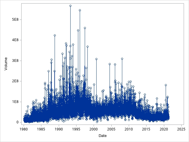
Firstly, I imported the data and gave the date variable a format that the program could read. This is important such that when we plot our graphs they are easier to read as it will show the exact date for each point instead of some arbitary number. After this, I plotted the data on a time series plot to visualise the data. From this plot I saw that the variance increased over time quite dramatically. This meant I then took a new variable called “logvolume” which is the logarithm of the volume variable to make the variance constant through out the time series plot.
proc sgplot data = intel_stock;
series x = Date y = logvolume/markers;
xaxis values = (1 to 5000 by 1);
run;
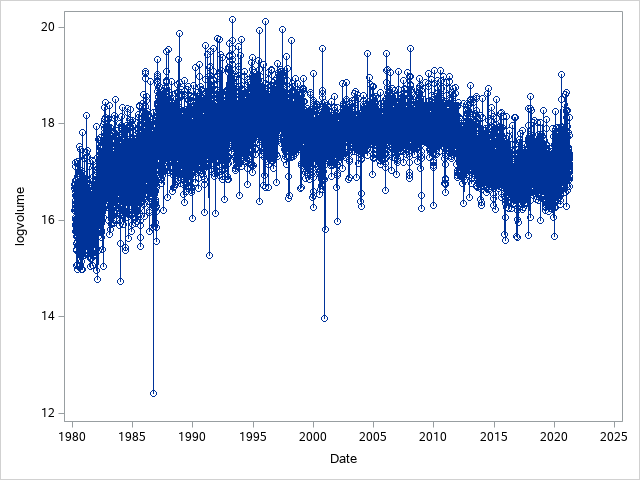
The plot shows a how the variance has been made constant by taking the logarithm of volume. We can also see two significant outliers that are resolved later. The plot however, shows that there is a non-zero mean.
Building and optimising a ARIMA model
proc arima data = intel_stock plots = all;
identify var= logvolume(1);
estimate p = 5 q = 5;
outlier id=Date;
run;
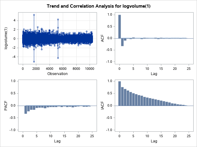
Now that I have obtained a time series with constant variance I need to make it stationary and that I need the mean of the model to be zero. We can do this by taking the first-difference of the variable logvolume. I then obtained the ARIMA plots using the code above to check if taking the first-difference worked. Using trial and error I found the best model with the lowest AIC was an ARIMA(5,1,5) model (AIC = 9392.761); residual correlation analysis suggests that model is a good fit for the data with now significant residuals in either the ACF or PACF plots. However, the model could be improved by identifying and resolving outliers.
.png)
The observation against logvolume(1) plot shows us the effect of taking the first-difference, we can clearly see that the mean is zero and thus we have obtained a stationary time series and can move onto building an ARIMA model. Firstly, I must identify and resolve any outliers; using outlier id=Date; we can identify any outliers by their date. Using this I identified 5 significant outliers:
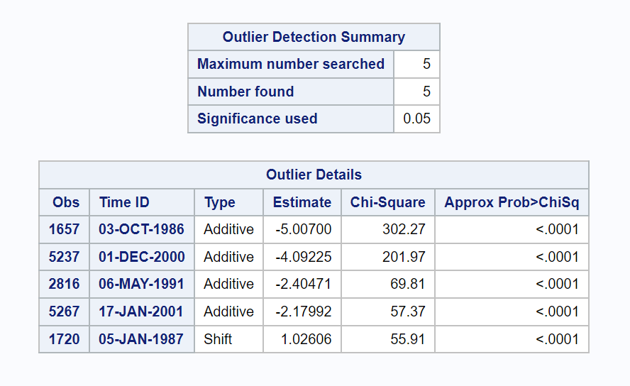
The code below attempts to resolve the outliers identified:
data intel_stock;
set intel_stock;
if _n_ = 1657 then AO = 1;
else AO = 0.0;
if _n_ = 5237 then AO = 1;
else AO = 0.0;
if _n_ = 2816 then AO = 1;
else AO = 0.0;
if _n_ >= 1720 then LS = 1;
else LS = 0.0;
if _n_ = 5267 then AO = 1;
else AO = 0.0;
run;
Code for the ARIMA plots:
proc arima data=intel_stock;
identify var=logvolume(1)
crosscorr=( AO(1) LS(1) );
estimate p = 5 q = 5 noint
input=( AO LS )
method=ml plot;
outlier id=Date;
run;
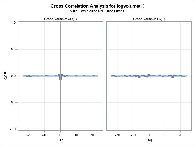

.png)
With the outliers resolved the model is already looking better. The AIC of this model is lower than the model with the outliers present (AIC = 9266.804), and the plot of white noise against lag shows overall a lower white noise probability suggesting that this model is better. Next I looked at the residual normality diagnostics.

Not much has changed in these plots compared to the previous model. Distribution of residuals seems to follow normal distribution quite nicely and the QQ-Plot shows us must points lay on the diagonal line suggesting normality. Since we have now optimised our model and obtained the lowest AIC possible we can now forecast accurately.
Forecasting and conclusions
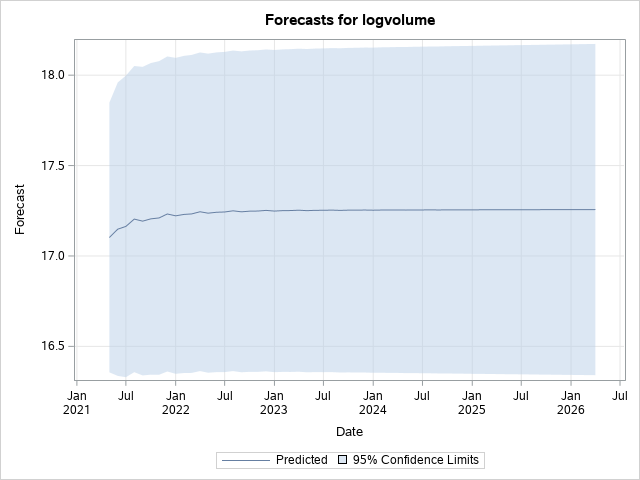

These plots show the forecast for the logvolume of the next 5 years. We see a small incline and then the curve flattens out, this is typical of an ARIMA model with no seasonality and the first-difference being taken. However, we cannot produce this graph to any clients or investors as it is still not a good visualisation of the forecast as we have just forecasted the logvolume, we do not care about the forecast for logvolume we wanted the forecast for the volume of stock. Hence, we alter our code and remove the logarithm by finding the exponential of our forecasted data.
data intel_forecast;
set forecast;
Volume = exp(logvolume);
l95 = exp(l95);
u95 = exp(u95);
forecast = exp(forecast + std*std/2);
run;
Now that the forecasts are in terms of the numbers of volume I was initially dealing with we can finally get a visualisation of the forecast with our original dataset. Using the code below produces a plot of the forecast with the original dataset.
proc sgplot data=intel_forecast;
where date >= '1JAN18'D;
band Upper=u95 Lower=l95 x=Date
/ legendLabel="95% Confidence Limits" ;
scatter x=Date y=Volume;
series x=Date y=forecast
/ legendlabel="Forecast of Volume for the next 5 years";
run;

The plot shows the forecast for the next 5 years for Intel’s volume of stock. I made a cut off point for any data before 2018 so that the forecast was more easily readable. From this forecast investors will easily be able to make a decision on buying stock, it is unlikely that the volume will decrease over the next 5 years. Infact, the 95% Confidence Limits suggest that on average the volume is more likely to be higher than forecasted than lower. The forecasts can also be used to predict the amount of storage needed, it is likely that Intel will need room for atleast 20,000,000 units whilst at most needing room for 75,000,000 units.